Want to share your content on R-bloggers? click here if you have a blog, or here if you don't.
What does marathon pacing data reveal about race strategy? Using R to analyze a comprehensive dataset of marathon finish times, we can uncover patterns in how runners manage their effort across 42.2 kilometers.
The gold standard for marathon pacing is the "even split"—maintaining identical pace from start to finish. Negative splitting, where you accelerate in the latter stages, remains largely the domain of elite athletes rather than recreational runners. The challenge with even-splitting lies in accurately gauging sustainable pace. After 30 kilometers, fatigue becomes universal, making slowdowns nearly unavoidable. Start too aggressively, and you'll experience the dreaded fade—what's known as "positive splitting."
Predicting maintainable marathon pace proves difficult despite tools like half-marathon time conversions. The marathon's punishing nature means training cycles require substantial time, recovery periods are lengthy, and running full-distance pace efforts during preparation is generally inadvisable. Determining optimal pace involves considerable estimation.
We analyzed chip-timed data from the 2025 New York City Marathon to understand real-world pacing patterns. The course profile features comparable first and second halves, making it ideal for examining split strategies. You can access the code to replicate this analysis.
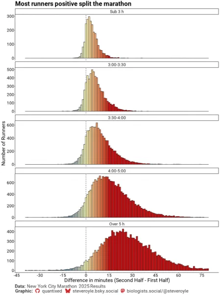
Histograms comparing first and second half times reveal that positive splitting dominates. Negative splitters (blue bars, left of the dashed line) represent a small minority. Even-splitters (yellow) are more common but still outnumbered by positive splitters (red).
Sub-3-hour finishers show a modal split of just +2 minutes—only 6 seconds per kilometer slower in the second half. For runners finishing beyond 5 hours, the fade extends to 20 minutes or more. While this suggests superior pacing discipline among faster runners, the pattern may simply reflect proportional slowdown relative to base pace.
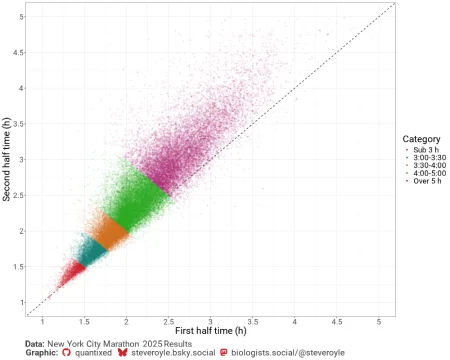
Plotting first-half versus second-half times directly confirms the scarcity of negative and even splits. Most runners cluster in the upper left quadrant, indicating positive splits. The data diverges from the ideal even-split line (dashed) in a linear fashion as pace slows.
Fitting a linear model constrained through the point (1,1)—representing a 2-hour even-split—using lm(formula = I(y - 60) ~ I(x - 60) + 0, data = fitting) yields a coefficient of 1.24. This represents the fade coefficient for the average 2025 NYC Marathon runner.
Practical application: A runner completing the first half in 90 minutes would likely finish the second half in 60 + 1.239 × (90 - 60) = 97.17 minutes, for a total time of 3:07:10.
For a 3-hour target, the average runner should aim for a first half of 60 / 2.239 + 60 = 86.8 minutes (1:26:48), anticipating a second half of 1:33:12.
Alternatively, calculating the mean ratio between half times across all finishers produces a fade coefficient of 1.13. This unconstrained approach suggests an 88-minute first half for 3-hour aspirants. Both coefficients provide reliable predictions across various finish times and likely apply to marathons with similar elevation profiles. Use these to calculate target pacing for your goal time.
For precision on sub-3-hour pacing, examining runners who finished between 2:50:00 and 3:00:00 reveals a median first half of 86.3 minutes (IQR: 84.4–87.87) and second half of 89.62 minutes (88.07–91.12), yielding a median finish of 2:56:00. A first-half time of 1:26:18 maximizes the probability of breaking 3 hours while accounting for inevitable fade.
The critical insight: abandon even-split assumptions when targeting a finish time. Aiming for 3:30:00 with 90-minute halves (4:59/km pace) sets you up for failure. Build in a buffer for the fade. Target 4:45/km instead (see table below).
Good luck!
| Finish Time | Even split pace | Target pace |
| 03:00:00 | 00:04:16 | 00:04:07 |
| 03:30:00 | 00:04:59 | 00:04:45 |
| 04:00:00 | 00:05:41 | 00:05:23 |
| 04:30:00 | 00:06:24 | 00:06:01 |
| 05:00:00 | 00:07:07 | 00:06:39 |
| 06:00:00 | 00:08:32 | 00:07:55 |
The code
This analysis was made possible by publicly available chip-time data. Thanks to Nicola Rennie for sharing techniques for styling social media handles in {ggplot2} graphics. The code includes my {qBrand} library for styling—skip this dependency by removing the caption = cap argument from ggplot calls.
The Code: Analyzing 2025 NYC Marathon Split Data
The analysis draws on split-time data for all 56,480 finishers of the 2025 New York City Marathon, sourced from a public dataset on Hugging Face. The R code below loads that CSV, extracts halfway and finish times, computes each runner's second-half split, and visualizes the results as both a faceted histogram and a scatter plot.
library(ggplot2)
library(ggtext)
sysfonts::font_add_google("Roboto", "roboto")
showtext::showtext_auto()

## data wrangling ----
url <- paste0("https://huggingface.co/datasets/donaldye8812/",
              "nyc-2025-marathon-splits/resolve/main/",
              "nyrr_marathon_2025_summary_56480_runners_WITH_SPLITS.csv")
df <- read.csv(url)

df <- df[df$splitCode %in% c("HALF", "MAR"), c("RunnerID", "splitCode", "time")]
df <- reshape(df, idvar = "RunnerID", timevar = "splitCode", direction = "wide")

df$split_HALF <- as.numeric(as.difftime(df$time.HALF, format = "%H:%M:%S", units = "mins"))
df$split_MAR  <- as.numeric(as.difftime(df$time.MAR,  format = "%H:%M:%S", units = "mins"))
df$split_SECOND_HALF <- df$split_MAR - df$split_HALF
df <- df[!is.na(df$split_SECOND_HALF), ]

df$Difference          <- df$split_SECOND_HALF - df$split_HALF
df$Difference_Fraction <- df$Difference / df$split_HALF * 100

df$Category <- cut(df$split_MAR,
                   breaks = c(0, 180, 210, 240, 300, Inf),
                   labels = c("Sub 3 h", "3:00-3:30", "3:30-4:00", "4:00-5:00", "Over 5 h"))

## plot styling ----
social    <- qBrand::qSocial()
cap       <- paste0("**Data:** New York City Marathon 2025 Results<br>**Graphic:** ", social)
my_palette <- c("Sub 3 h"   = "#cb2029",
                "3:00-3:30" = "#147f77",
                "3:30-4:00" = "#cf6d21",
                "4:00-5:00" = "#28a91b",
                "Over 5 h"  = "#a31a6d")

## histogram ----
ggplot(df, aes(x = Difference, fill = after_stat(x))) +
  geom_vline(xintercept = 0, linetype = "dashed", color = "black") +
  geom_histogram(breaks = seq(from = -59.5, to = 81.5, by = 1), color = "black") +
  scale_colour_gradient2(
    low = "#2b83ba", mid = "#ffffbf", high = "#d7191c",
    midpoint = 0, limits = c(-15, 15), na.value = "#ffffffff",
    guide = "colourbar", aesthetics = "fill", oob = scales::squish
  ) +
  scale_x_continuous(breaks = seq(-45, 90, 15), limits = c(-40, 80)) +
  facet_wrap(~ Category, ncol = 1, scales = "free_y") +
  labs(title = "Most runners positive split the marathon",
       x = "Difference in minutes (Second Half – First Half)",
       y = "Number of Runners",
       caption = cap) +
  theme_classic() +
  theme(
    legend.position = "none",
    plot.caption = element_textbox_simple(
      colour = "grey25", hjust = 0, halign = 0,
      margin = margin(b = 0, t = 5), size = rel(0.9)
    ),
    text       = element_text(family = "roboto", size = 16),
    plot.title = element_text(size = rel(1.2), face = "bold")
  )

ggsave("Output/Plots/nyc_marathon_2025_split_difference_histogram.png",
       width = 900, height = 1200, dpi = 72, units = "px", bg = "white")

## scatter plot ----
ggplot() +
  geom_abline(slope = 1, linetype = "dashed", color = "black") +
  geom_point(data = df,
             aes(x = split_HALF, y = split_SECOND_HALF, colour = Category),
             shape = 16, size = 1.5, alpha = 0.1) +
  scale_x_continuous(breaks = seq(0, 12 * 30, 30),
                     labels = seq(0, 6, 0.5),
                     limits = c(60, 300)) +
  scale_y_continuous(breaks = seq(0, 12 * 30, 30),
                     labels = seq(0, 6, 0.5),
                     limits = c(60, 300)) +
  scale_colour_manual(values = my_palette) +
  labs(x = "First half time (h)", y = "Second half time (h)", caption = cap) +
  theme_bw() +
  theme(
    plot.caption = element_textbox_simple(
      colour = "grey25", hjust = 0, halign = 0,
      margin = margin(b = 0, t = 10), size = rel(0.9)
    ),
    text = element_text(family = "roboto", size = 16)
  ) +
  guides(colour = guide_legend(override.aes = list(alpha = 1)))

ggsave("Output/Plots/nyc_marathon_2025_split_difference_scatter.png",
       width = 1000, height = 800, dpi = 72, units = "px", bg = "white")
From this data we can also derive some useful pacing benchmarks through linear regression.
## fitting ----
# Constrain the regression line through (60, 60) — representing a 2-hour
# marathoner running perfectly even splits
fitting <- data.frame(x = df$split_HALF, y = df$split_SECOND_HALF)
lm(I(y - 60) ~ I(x - 60) + 0, data = fitting)

# Coefficients:
#   I(x - 60)
#       1.239

# Interpretation: for a 90-minute first half, the model predicts a second half of:
# 60 + 1.239 × (90 − 60) = 97.17 minutes → finish time of 3:07:10
#
# To target a sub-3-hour finish at NYC, the average runner would need to run:
# 60 / 2.239 + 60 = 86.8 minutes for the first half (1:26:48),
# leaving 1:33:12 for the second half.

# A simpler measure: the mean second-half / first-half ratio across all finishers
mean_ratio <- mean(df$split_SECOND_HALF / df$split_HALF)
mean_ratio
# [1] 1.127581

# Zooming in on sub-3-hour finishers (finish time between 170 and 180 minutes)
target <- df[df$split_MAR > 170 & df$split_MAR < 180, ]
summary(target)

#    RunnerID       time.HALF          time.MAR          split_HALF      split_MAR     split_SECOND_HALF   Difference
#  Min.   :48819892   Length:1289   Length:1289   Min.   :70.25   Min.   :170.0   Min.   : 82.70   Min.   :-7.6833
#  1st Qu.:48834548   Class :character             1st Qu.:84.42   1st Qu.:173.6   1st Qu.: 88.07   1st Qu.: 0.7167
#  Median :48849752   Mode  :character             Median :86.30   Median :176.0   Median : 89.62   Median : 3.0500
#  Mean   :48849498                                Mean   :85.98   Mean   :175.7   Mean   : 89.73   Mean   : 3.7585
#  3rd Qu.:48864551                                3rd Qu.:87.87   3rd Qu.:178.2   3rd Qu.: 91.12   3rd Qu.: 5.9000
#  Max.   :48878979                                Max.   :92.87   Max.   :180.0   Max.   :106.02   Max.   :35.7667
#
#  Difference_Fraction   Category
#  Min.   :-8.5008       Sub 3 h :1289
#  1st Qu.: 0.8051       3:00-3:30:   0
#  Median : 3.5390       3:30-4:00:   0
#  Mean   : 4.5178       4:00-5:00:   0
#  3rd Qu.: 7.0055       Over 5 h :   0
#  Max.   :50.9134
The post title is a nod to "Marathon Man" by Ian Brown, from his album My Way — though the tracksuit he's wearing on the cover is decidedly not race-day attire.
R-bloggers.com offers daily e-mail updates about R news and tutorials about learning R and many other topics. Click here if you're looking to post or find an R/data-science job.
Want to share your content on R-bloggers? Click here if you have a blog, or here if you don't.
Continue reading: Marathon Man: how to pace a marathon